Anomaly Detection Model Overview
211 call counts and five high-level features
What 211 Calls Are
United Way 211
United Way 211 is a community referral system that connects people to services and support.
Examples include:
- food insecurity and meal resources
- housing and utility assistance
- mental health and crisis support
- transportation and other basic-needs services
Why these calls matter
Changes in 211 calls can reflect changing community needs, access problems, or acute events.
This talk focuses on 211 counts related to food insecurity and meal resources.
211 Background
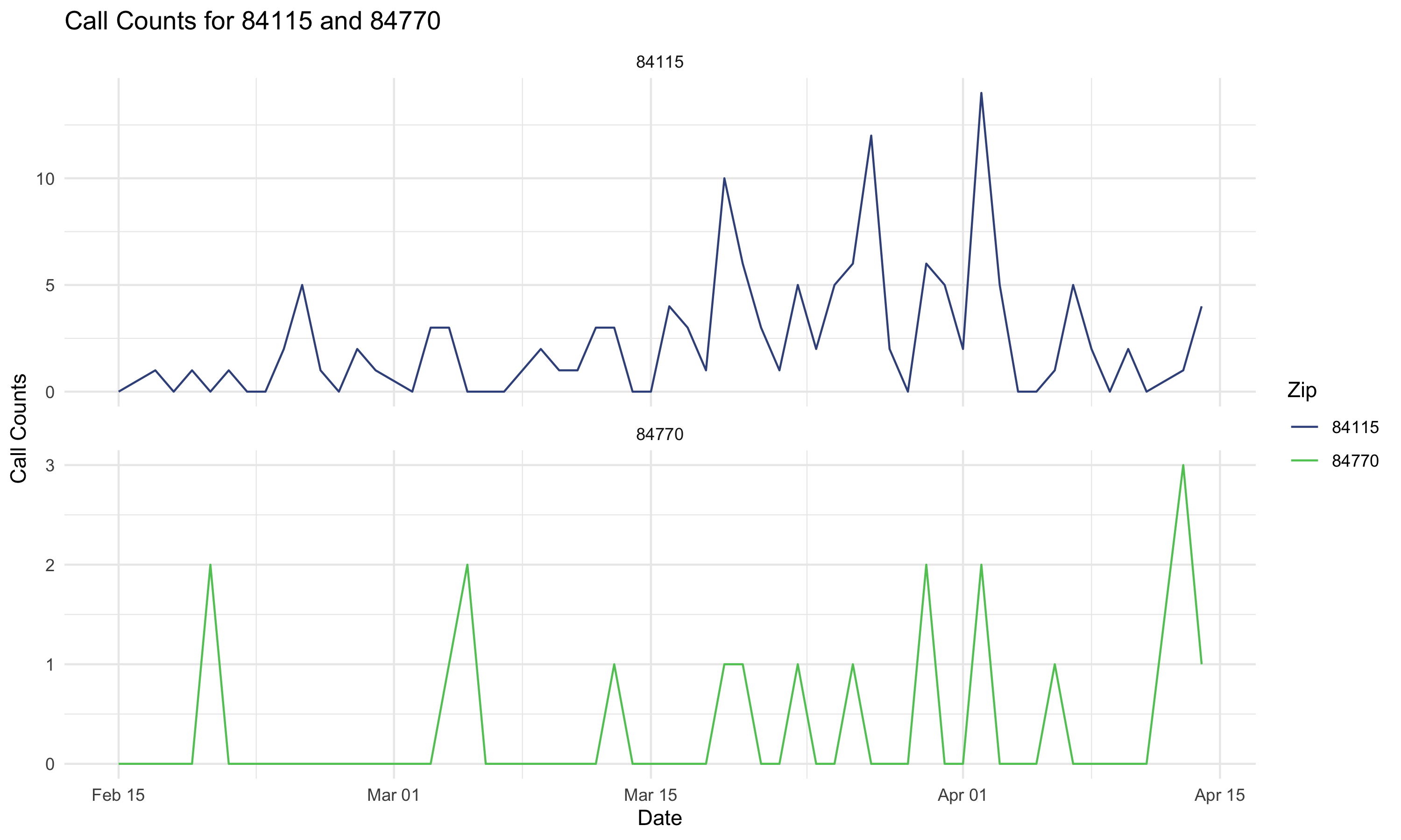
Why 211 counts are hard to interpret visually
Daily 211 call counts move for a lot of reasons:
- Low call counts
- weekly usage patterns
- seasonality across the year
- gradual changes in underlying demand
- sudden events that create real spikes
What we want
We want to distinguish the expected pattern from signals that may matter operationally.
Why A Model Is Helpful
The goal is not just to find high-count days.
The goal is to find days that are unusually high after accounting for the normal structure in 211 call counts.
The next slide is the main navigation slide. Each feature can be clicked to jump into a backup slide, and each backup slide links back here.
Five High-Level Features
Sparse series and overdispersed counts.
Rate jumps, ramp selection, and anomalies.
Weekday effects in both counts and zero inflation.
Recurring seasonal patterns across the year.
Nearby days can move together.
Spatial structure, trend changes, and computation.
Feature 1: Many Zeros And Flexible Count Data
Main idea
211 series can include many zeros in some settings, and count variability can exceed what a simple Poisson model would allow.
Why that matters
- the model can accommodate sparse count series
- it is flexible for overdispersed count data
- this makes the framework more useful across very different call settings
Feature 1 Code: Many Zeros And Flexible Count Data
vector<lower=0>[C] inv_phi;
vector[C] h0;

phi[c] = 1 / inv_phi[c];
logit_zi[c][t] = h0[c] + eta[c][dow[t]];

if (y[c, t] == 0) {
  target += log_mix(inv_logit(logit_zi[c][t]),
                    0,
                    neg_binomial_2_log_lpmf(0 | log_lambda[c][t], phi[c]));
} else {
  target += bernoulli_logit_lpmf(0 | logit_zi[c][t])
            + neg_binomial_2_log_lpmf(y[c, t] | log_lambda[c][t], phi[c]);
}Feature 2: Rate Jumps, Ramp Selection, And Anomalies
Main idea
The model can represent abrupt changes in the underlying rate, allows multiple smooth ramps, and uses a separate anomaly channel for local departures.
Why that matters
- sustained jumps in the rate are not forced into one-day spike terms
- the model can adapt to more than one structural change over time
- local anomalies can still be highlighted after those broader changes are accounted for
Feature 2 Code: Rate Jumps, Ramp Selection, And Anomalies
vector[J] tau_raw = sort_asc(inv_logit(tau_unconstrained[c]));
for (j in 1:J) {
  tau[c][j] = 1 + (T - 1) * tau_raw[j];
  s[c][j]   = exp(log_s[c][j]);
}
d[c] = d_raw[c] .* lambda[c] * hs_tau[c];
kappa[c] = sigma_kappa[c] * kappa_raw[c];

for (t in 1:T) {
  real ramps = m0[c];
  for (j in 1:J) {
    ramps += d[c][j] * inv_logit((t - tau[c][j]) / s[c][j]);
  }
  log_lambda[c][t] = ramps + gamma[c][dow[t]] + z[c][t] + kappa[c][t] + season[c][t];
}Feature 3: Day-Of-Week Effects
Main idea
211 activity differs systematically across the week, so the model includes day-of-week effects in both the count part of the model and the zero-inflation part.
Why that matters
- routine weekday differences are not mistaken for meaningful events
- comparisons across days become fairer
- the chance of observing zeros can also vary by weekday
Feature 3 Code: Day-Of-Week Effects
array[C] vector[6] gamma_raw;
array[C] vector[7] gamma;
array[C] vector[6] eta_raw;
array[C] vector[7] eta;

gamma[c][1:6] = gamma_raw[c];
gamma[c][7]   = -sum(gamma_raw[c]);
eta[c][1:6] = eta_raw[c];
eta[c][7]   = -sum(eta_raw[c]);

for (t in 1:T) {
  logit_zi[c][t] = h0[c] + eta[c][dow[t]];
  log_lambda[c][t] = ramps + gamma[c][dow[t]] + z[c][t] + kappa[c][t] + season[c][t];
}Feature 4: Seasonality
Main idea
The model includes a seasonal component so recurring patterns across the year aren’t identified as anomalies.
Why that matters
- predictable seasonal shifts are absorbed before detection decisions
- anomalies are judged relative to the expected time of year
- this is especially useful when call patterns drift across seasons
Feature 4 Code: Seasonality
Feature 5: AR(1) Correlation
Main idea
Nearby days are allowed to be correlated through an AR(1) structure, rather than assuming each day is independent after adjustment.
Why that matters
- short runs of elevated or depressed counts are modeled more realistically
- the model is less likely to overreact to small clusters of related days
- residual structure is separated from truly unusual single-day behavior
Feature 5 Code: AR(1) Correlation
Future Features And Issues
Main idea
Two natural extensions are:
- a spatial component so nearby counties or ZIPs can share information
- more flexible trend changes so the model can represent evolving slopes, not only ramps
- a faster computational strategy for repeated fitting across Utah ZIP codes over time
Why that matters
- spatial borrowing could stabilize estimates in sparse areas
- neighboring regions may show related patterns during shared events
- trend-change components could capture gradual accelerations or slowdowns more naturally
- computational time becomes a real issue when fitting many ZIP codes repeatedly across rolling dates
Notes: Future Features And Issues
These are extensions rather than current features.
Possible directions
- add a spatial random effect or adjacency-based structure across counties or ZIPs
- replace or augment ramps with components that allow changes in slope over time
- combine those additions with the current anomaly channel rather than replacing it
- reduce runtime for statewide ZIP-level monitoring through approximation, parallelization, or a more scalable model structure
Why Stan Is Useful Here
Why implement this in Stan
This model combines several pieces at once:
- zero inflation and flexible count likelihoods
- smooth rate changes
- anomaly terms
- day-of-week effects
- seasonality
- AR(1) dependence
Stan makes it practical to estimate all of these pieces jointly in one coherent model.
Why that matters computationally
- Hamiltonian Monte Carlo is well suited for a rich continuous-parameter model
- uncertainty is propagated across all components together
- transformed-data tricks, vectorization, and non-centered parameterizations help with efficiency and stability
This would be much harder to fit well with ad hoc step-by-step estimation or with a frequentist approach.
Model Overview